Short-term Load Forecast

I know electric load forecasting might not be the sexiest sounding topic, but all of us are users of electricity and power companies really need to understand our consumption behavior at the aggregate level in order to serve us well. Imagine the complexities in this forecast problem.

We all have different schedules; we may have individually metered homes or some form of paying a portion of a shared bill; we may operate a small business that have very different usage profiles than someone who goes to a traditional workplace from 9 to 5. And here is the ultimate catch: Before large scale battery technology really catches on, there’s no good way to store energy produced. That means utilities need to produce exactly (roughly speaking) the amount that their customers need at any given moment. And let’s not even mention all kinds of seasonalities–well, I will in a bit.

1. Visualizing the Time Series

If you haven’t seen a load profile before, here is a picture for you.

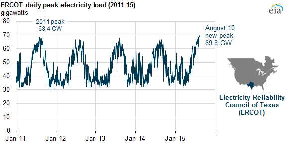
This somewhat dated graph shows the daily peak consumption for ERCOT (Electric Reliability Council of Texas) from our trusty Energy Information Agency. We see the repeating cyclical pattern here but also a lot of small wiggles along the way.

By the way, the forecast problem I’ll be attempting here is on a different time scale. Instead of the daily peak, I’ll be forecasting hourly consumption for a very short look-ahead period (24-48 hrs to 2 weeks at most). The different time scales do have business implications about the speed and availability of data, the allowable model training time, etc. But more importantly, we need training data to be of the same granularity as what we are trying to predict. Obviously, the finer the granularity, the larger the dataset that we’ll most likely be talking about.

2. Roadmap

Here are a few modeling approaches that I tried for this problem:

• classical time series approach, best typified by the sophisticated fbprophet package develped by Facebook
• decision tree model using weather forecast and appropriately lagged variables as features
• recurrent neural net that requires very small initial setup but needs long experimentation and training time to nail down good (enough) model with acceptable time/accuracy trade-off

a. Prophet

Once I’ve wrangled the input data into the form that Prophet requires, the fitting and predition steps are relatively straight forward.

m = Prophet()
m.fit(df)
future = m.make_future_dataframe(periods=24, freq='H')
forecast = m.predict(future)
forecast[['ds', 'yhat', 'yhat_lower', 'yhat_upper']].tail()

The underlying model is an aggregation of decomposed trend, seasonality and holiday components. Each one of these individual components has quite a bit of complexity underneath. The trend component admits change points (How does one find change points? You may ask.), the seasonality component can have multiple seasonalities embedded and disentangled, if you will, only by a Fourier series. The sum result is that the curve fitting is non-trivial and I found out the hard way that on large problem sets such as this (hourly input data over a number of years), the computer can chug along for quite a while doing the compute.

For anyone interested in the inner workings, definitely check out Facebook’s site on this tool

b. Decision Tree Regressor

To avoid using something that is a little black-boxy and janky at times, it’s easy to write up a tree-based model with some care applied to engineering the right features. Here, there is a some literature out there and I liberally borrowed ideas from this matlab post for solving a similar problem.

Eventually, the following variables were created in my case:

• hourly consumption of the previous day
• hourly consumption of the same day of the week the prior week
• previous day daily average
• time indicator variables such as hour of day, day of week, weekday/weekend flag, and possibly day of year

The above set is in addition to the weather variables that would have been made available at the time of the load forecast, the most important of which are dry bulb temperature and humidity.

c. RNN

Where’s the fun if we didn’t experiment with recurrent neural net? This class of prediction prolem, of which weather forecast itself is a cannonical example, lends naturally to this approach, although implementation (using generator when doing the batch processing) and model selection (playing with different architectures of layers and hidden units) may be too much of a chore to go through for business cases that can be well-served by the more explainable models in the prior sections. Not to mention that if the training time involved for RNN is on the scale of hours instead of minutes, the forecast itself may be stale before it even becomes available.

Regardless, I find the exercise illuminating if not for practising keeping track of things especially in a generator context:

def generator(data, lookback, delay, min_index, max_index,
              shuffle=False, batchsize=168, step=1):
    if max_index is None:
        max_index = len(data) - delay - 1
    i = min_index + lookback
    while 1:
        if shuffle:
            rows = np.random.randint(min_index + lookback, max_index, size=batchsize)
        else:
            if i + batchsize >= max_index:
                i = min_index + lookback
            # np.arange(start, stop(not including))
            rows = np.arange(i, min(i + batchsize, max_index))
            i += len(rows)
        samples = np.zeros((len(rows),
                           lookback//step,
                           data.shape[-1]))
        targets = np.zeros(len(rows), )
        for j, row in enumerate(rows):
            indices = range(rows[j] - lookback, rows[j], step)
            samples[j] = data[indices]
            targets[j] = data[rows[j] + delay][0]
        yield samples, targets

Just for illustration, this is the final neural network architecture that I chose, with the loss function modified to get forecast of quantiles for boudning the uncertainty.

def tilted_loss(q,y,f):
    e = (y-f)
    return K.mean(K.maximum(q*e, (q-1)*e), axis=-1)

def build_rnn():
    model = models.Sequential()
    model.add(layers.Conv1D(32, 5, activation='relu',
                            input_shape=(None, train_data.shape[-1])))
    model.add(layers.MaxPooling1D(3))
    model.add(layers.Conv1D(32, 5, activation='relu'))
    model.add(layers.GRU(32))
    model.add(layers.Dense(1))
    model.compile(optimizer='rmsprop', loss=lambda y,f: tilted_loss(quantile,y,f), metrics=['mae'])
    return model

quantile = 0.5
model_rnn = build_rnn()
model_rnn.summary()

history_rnn = model_rnn.fit_generator(train_gen,
                                      steps_per_epoch=365,
                                      epochs=20,
                                      validation_data=val_gen,
                                      validation_steps=50,
                                      callbacks = [
                                          callbacks.ReduceLROnPlateau(factor=.5, patience=3, verbose=1)
                                      ])
test_metrics_rnn = model_rnn.evaluate_generator(test_gen, steps=10)

3. Performance

As I used the RNN model to forecast 2 weeks, the model did not have the benefit of having usable weather forecast information. It is not surprising that the MAPE (mean absolute percent error) over a one year test set is around 10% (shown below for a one week period with 95% prediction interval and against actual), versus 5% of the decision tree model.

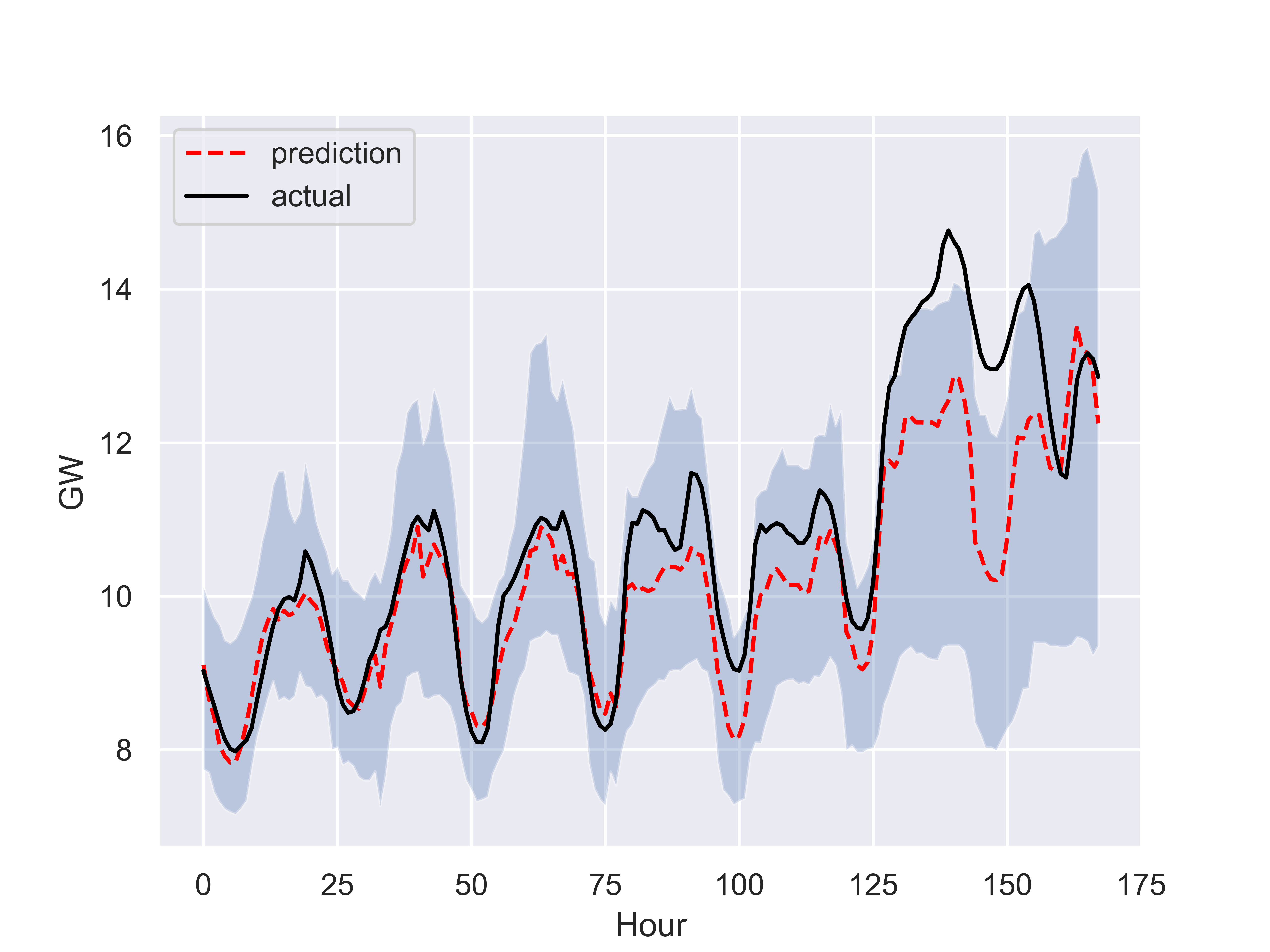
Both models lose quite a bit of accuracy toward the end of the period shown (even though the decision tree regressor catches up with actual data on a daily basis) as the test location experienced an unprecedented cold snap for a couple of days. I guess nothing says predictions are only as good as what past data can teach you as well as this snapshot.