Life and Death Classification
One of the more “insightful” projects that I did during my Metis program is a scaled-down version of Kaggle’s pet adotpion competition. link here
While not personally owner of any furry friends, I’ve always had a yearning to break down the cute facade of house pets (in this case, dogs) and see what lies beneath! Alas, cuteness comes in many flavors and is more in the eye of the beholder so the project turns out to be a good education of what people value in dogs at least as they make their decision to adopt (or not).
The rather unsavory fact was never too far off in the background, however, that if shelter animals stay in the shelter beyond a certain number of days without adoption, they are most likely destined for a tragic end–there are millions of stray pets being euthanized every year just in the United States. A life-and-death situation indeed.
1. A Much Simplified Data Processing Step
To keep the project feasible within the time constraint, I chose to ignore the photo collection keyed to the individual pet ID’s. A few pets with missing profile sentiment analysis were dropped. And instead of a multi-class classficication of how soon an adoption occurs (1 month, 2 months, etc.), a binary target of whether adopted within 100 days (the longest timeframe in the data) was created.
# keep only the records that have sentiment score
train_df = train_df.merge(train_sent, how='inner', left_on='PetID', right_index=True)
train_df['AdoptionSpeed'] = train_df['AdoptionSpeed'].replace({1: 0, 2: 0, 3: 0, 4: 1})
2. Model Baselining and Feature Engineering
After some preliminary EDA,
def plot_features(df):
    sample = df[numeric_cols].sample(1000, random_state=44)
    sns.pairplot(sample, hue='AdoptionSpeed', plot_kws=dict(alpha=.3, edgecolor='none'))
I proceded to use a logistic regression model as the baseline, paying attention to the features that have “large” effects. This will become more interesting when I tested out tree-based models later and plotted out features by importance. As in the latter instance, the direction of influence is not known, only the degree of information gain.
feature_coefs = pd.DataFrame({'feature': feature_names, 'coef': logit.coef_[0]})
feature_coefs['abs_coef'] = abs(feature_coefs['coef'])
feature_coefs.sort_values(by='abs_coef', ascending=False, inplace=True)
To supplement the given dataset, I scraped the wikipedia page (struggling mightily with encoding) where breed names are mapped to the breed groups as stipulated by the American Kennel Club (eg., hound, terrier, sporting, herding, toy, etc.). AKC keeps a database that shows the personalities of each individual breed. However, aggregating at the breed group level gives a good approximation of the effect of breed on adoption.
import unicodedata
breed_groups = pd.read_csv('data/breed_groups.csv', encoding='latin_1')
for i in range(len(breed_groups['BreedName'])):
    breed_groups['BreedName'][i] = unicodedata.normalize('NFKD', breed_groups['BreedName'][i]).\
        encode('ascii', 'ignore').decode('utf-8')
3. Performance Measurement
Venturing onto tree-based models, I started off with random forest, then tried extreme trees and adaboost. Not having any clear winner, I experimented with stacking these models. It’s not surprisng perhaps that stacking these similar models didn’t provide any performance boost. Presumably, when one of the tree models got it wrong, the others did too.
Even though I used the f1 score when comparing across different models, it’s good to keep an eye on things like the confustion matrix
confusion = confusion_matrix(label_test_s, rfmodel_fin.predict(Xs_test))
plt.figure(dpi=150)
sns.heatmap(confusion, cmap=plt.cm.Blues, annot=True, square=True, fmt='g',
            xticklabels=['adopted', 'not adopted'],
            yticklabels=['adopted', 'not adopted'])
plt.xlabel('Predicted Adoptions')
plt.ylabel('Actual Adoptions')
plt.show()
… and the ROC AUC.
fpr, tpr, thresholds = roc_curve(label_test_s, rfmodel_fin.predict_proba(Xs_test)[:, 1])
plt.plot(fpr, tpr, lw=2)
plt.plot([0, 1], [0, 1], c='violet', ls='--')
plt.xlim([-0.05, 1.05])
plt.ylim([-0.05, 1.05])
plt.xlabel('False positive rate')
plt.ylabel('True positive rate')
plt.title('ROC curve for pet adoption')
plt.show()
print("ROC AUC score = ", roc_auc_score(label_test_s, rfmodel_fin.predict_proba(Xs_test)[:, 1]))
As mentioned, stacking some tree models and using metaclassifier didn’t improve the score.
models = ['rf', 'et', 'adb']
for model_name in models:
    curr_model = eval(model_name)
    curr_model.fit(Xs_train, label_train_s)
    print(f'{model_name} score: {f1_score(label_test_s, curr_model.predict(Xs_test))}')

stacked = StackingClassifier(classifiers=[eval(n) for n in models],
                             meta_classifier=BernoulliNB(),
                             use_probas=False)
stacked.fit(Xs_train, label_train_s)
print(f'stacked score: {f1_score(label_test_s, stacked.predict(Xs_test))}')
xgboost in conjuction with GridSearchCV did outperform the previous models but with the added complication that since the package doesn’t include a native method to correct for class imbalance (as was the case with the class_weight option for logistic regression and random forest in sklearn), I had to use the RandomOverSampler from the imblearn package.
fin_model = xgb.XGBClassifier(objective='binary:logistic')
params = {
    'n_estimators': [100, 200],
    'min_child_weight': [1, 3],
    'gamma': [0.5, 1],
    'subsample': [0.8, 1.0],
    'colsample_bytree': [0.8, 1.0],
    'max_depth': [4, 5, 6],
    'learning_rate': [0.05, 0.1, 0.2, 0.3]
        }
grid_search = GridSearchCV(fin_model, params, scoring="f1", n_jobs=-1, cv=5)
grid_result = grid_search.fit(X_ros, y_ros)
4. Neural Network Attempt
I guess it doesn’t hurt to try the neural network approach, even though I could not be anywhere near exhaustive with it. Taking the same care about resampling due to class imbalance, internet comes to the rescue about using f1 as the custom scoring metric during model fitting and optimization.
def f1(y_true, y_pred):
    def recall(y_true, y_pred):
        """Recall metric.
        Only computes a batch-wise average of recall.
        Computes the recall, a metric for multi-label classification of
        how many relevant items are selected.
        """
        true_positives = K.sum(K.round(K.clip(y_true * y_pred, 0, 1)))
        possible_positives = K.sum(K.round(K.clip(y_true, 0, 1)))
        recall = true_positives / (possible_positives + K.epsilon())
        return recall

    def precision(y_true, y_pred):
        """Precision metric.
        Only computes a batch-wise average of precision.
        Computes the precision, a metric for multi-label classification of
        how many selected items are relevant.
        """
        true_positives = K.sum(K.round(K.clip(y_true * y_pred, 0, 1)))
        predicted_positives = K.sum(K.round(K.clip(y_pred, 0, 1)))
        precision = true_positives / (predicted_positives + K.epsilon())
        return precision
    precision = precision(y_true, y_pred)
    recall = recall(y_true, y_pred)
    return 2*((precision*recall)/(precision+recall+K.epsilon()))

def build_model():
    nn_model = keras.models.Sequential()
    nn_model.add(keras.layers.Dense(units=20, input_dim=X_ros_train.shape[1], activation='tanh'))
    nn_model.add(keras.layers.Dense(units=20, activation='tanh'))
    nn_model.add(keras.layers.Dense(units=1, activation='sigmoid'))

    nn_model.compile(loss='binary_crossentropy',
                     optimizer= "adam",
                     metrics=[f1])
    return nn_model

# create plot of loss/metric over epochs for training and validation
def plot_train_val_scores(model_h):
    score = model_h.history['f1']
    val_score = model_h.history['val_f1']
    history_dict = model_h.history
    epochs = range(1, len(history_dict['f1']) + 1)

    plt.plot(epochs, score, 'bo', label='training f1 score')  # blue dot
    plt.plot(epochs, val_score, 'b', label='validation f1 score')
    plt.title('training and validation f1 score')
    plt.xlabel('Epochs')
    plt.ylabel('f1')
    plt.legend()

nn_model = build_model()
h = nn_model.fit(X_ros_train, label_ros_train, batch_size=100, epochs=200,
                 validation_data=(X_ros_val, label_ros_val))
nn_model.evaluate(Xs_test, label_test_s)
Varying batch_size, epochs, layer number and hidden unit number will alter the results but neural nets ultimately didn’t win out given the limited tries. That they are so time-consuming is a vote against going beyond mere experimentation.
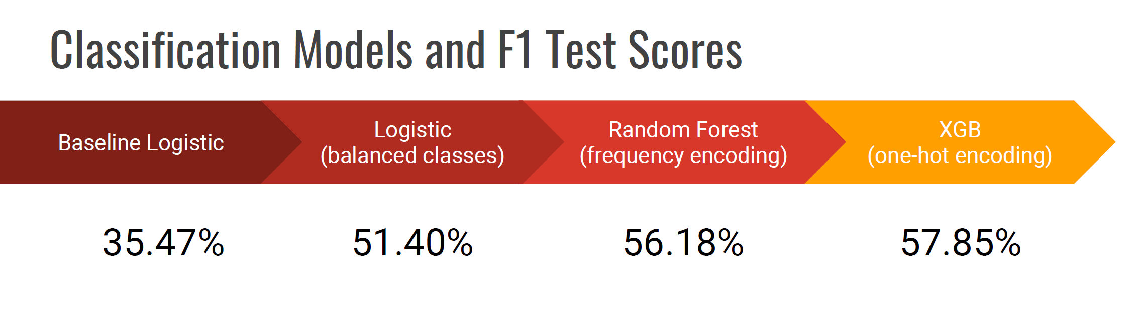
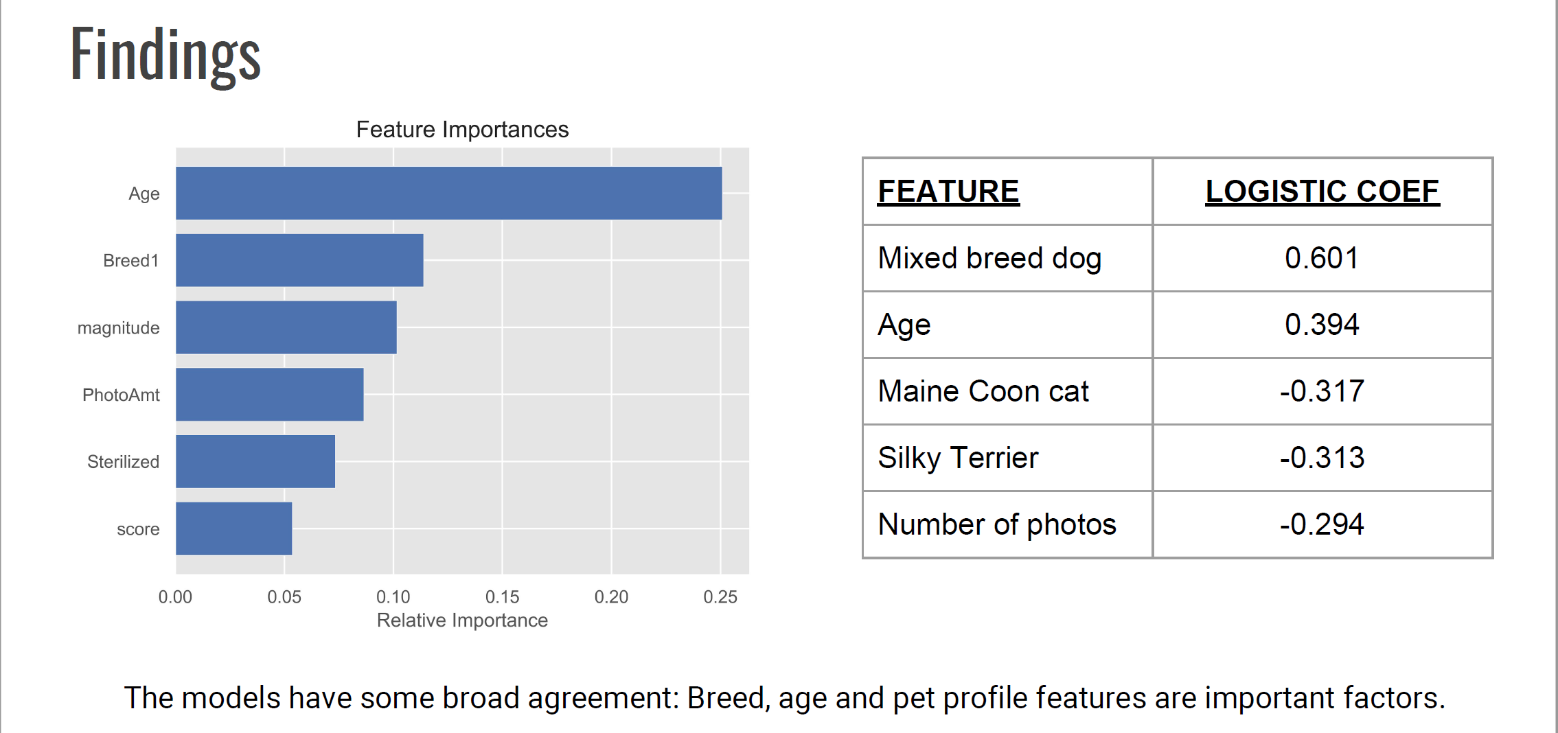
5. Conclusions
So what are the findings in terms of important features?
 And how do the models compare?